926
The VLOOKUP function in Excel makes it easier for you to search for specific values or elements within tables and other defined areas
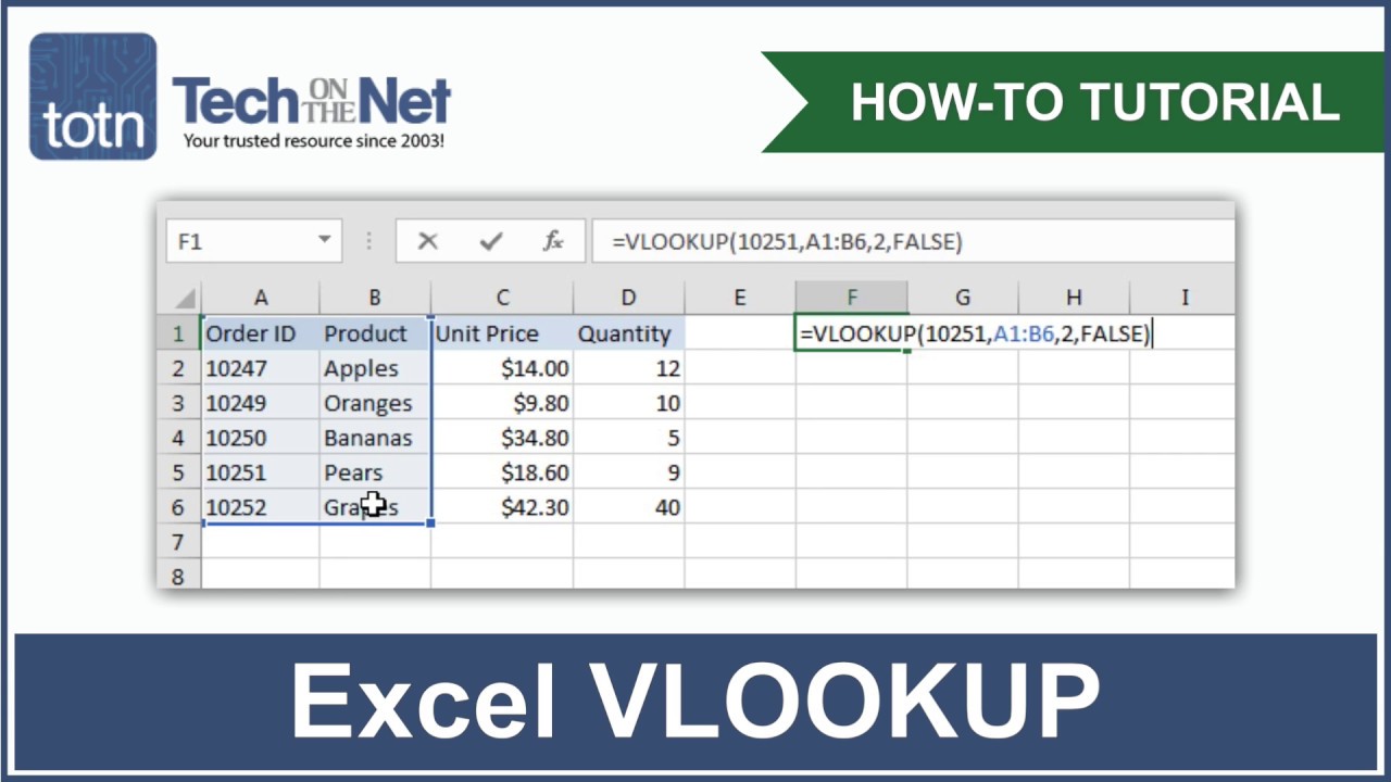
Excel VLOOKUP: Using the function
VLOOKUP allows you to automatically find specific values in Excel based on a search criterion you specify.
- The formula of the Excel function is as follows: =VLOOKUP(search criterion; matrix; column index; [range_reference])
- The search criterion is the field in the document, for example D3 or F10, in which you enter the search term. For example, if you have prepared a table with vehicle replacement lines and their location in the warehouse, enter the exact product in the search field.
- For the matrix, simply select the area of the table that you want to search. Make sure that you only select the values and not the table headings. This is displayed in the formula, for example, as A1:B80.
- Use the column index to specify the column as a number that the function should search for the value. In other words, the first column as 1, the second as 2 and so on.
- Two options are available for [Range_reference]. Use FALSE to search for the exact value and TRUE to search for the approximate value. The default setting is always TRUE
- Complete the formula. You can then enter the search criterion in the search field and the VLOOKUP function will show you the corresponding value.